Getting started¶

This quickstart will walk you through a minimal end-to-end example of how to use socca to model an astronomical image. In this specific example, we will model a simulated toy image of a disk-like galaxy using a model comprising a Sérsic component and a point source.

Image of a mock galaxy, comprising a Sérsic component and a point source.

You can access all the files you need to run this tutorial here.

Before getting into the nuts and bolts of using socca to model your favourite image, we first need to load socca:

>>> import socca

Ready, set, go!

Loading the data¶

As a first step, we build the data structure. The first element to define is the noise model, which is used by socca to determine the likelihood function for the inference. The simplest noise model (and the one injected in the mock data used here) assumes a normal distribution with statistically independent resolution elements (i.e. no pixel-to-pixel correlations). This can be defined as follows:

>>> noise = socca.noise.Normal()

When no arguments are passed, Normal is configured to infer the standard deviation of the noise distribution directly from the input image. This estimate is based on the median absolute deviation of the pixel values. It is also possible to manually specify the standard deviation, variance, or inverse variance (i.e. weight) of the distribution, either as constant values across the image or by providing a corresponding map (see the “Noise models” documentation page for more details).

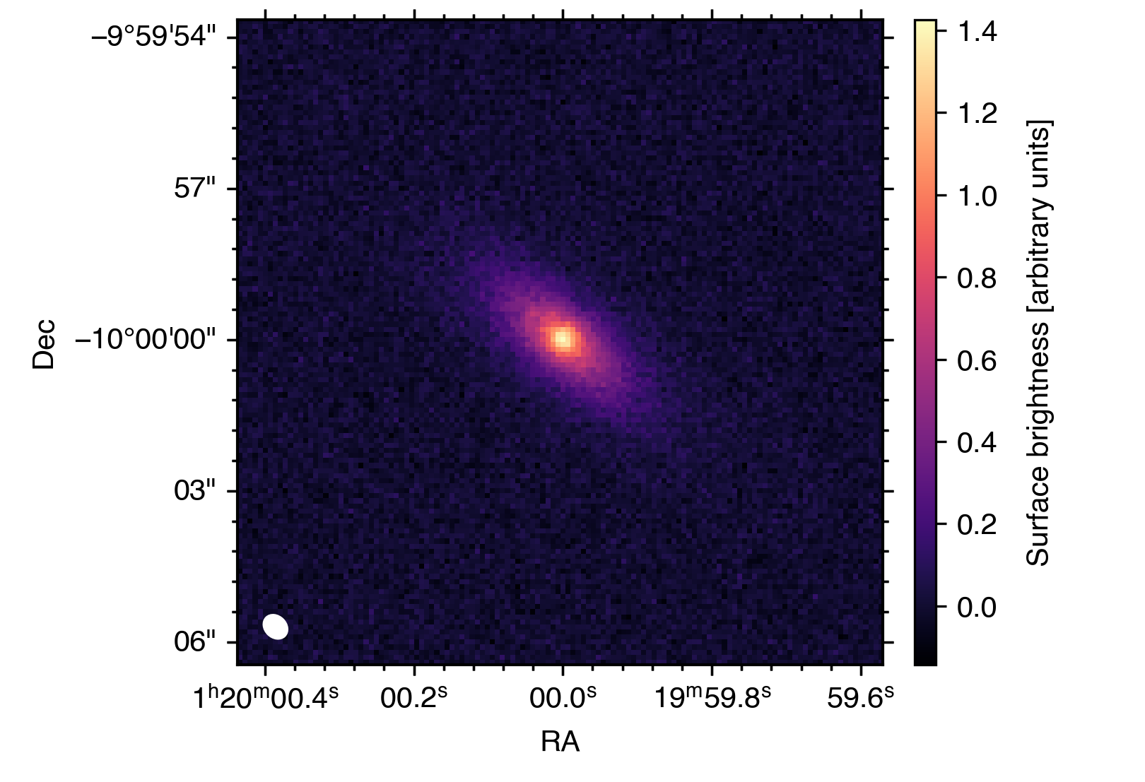
We are now ready to load the image (and let socca handle much of the associated bookkeeping):

>>> img = socca.data.Image(img='tutorial_mock.fits', noise=noise)
Using MAD for estimating noise level
- noise level: 4.47E-02

As mentioned above, socca uses the image itself to estimate the noise properties, measuring a root-mean-square noise level of 4.47×10^-2 (in image units).

Defining a model¶

The next step is to define a model for the astronomical source(s) we want to fit. The basic building blocks of any model in socca are individual modular components, which can be combined linearly to describe the complex morphology of astronomical sources.

Point source¶

As a first step, each component is defined independently and later combined into a single model. We start by defining a point-like component using the Point class from the socca.models module:

>>> point = socca.models.Point()

The point object now represents a point-like model component that can be used to describe unresolved sources. To inspect the parameters associated with this model, we can use the parameters() method:

>>> point.parameters()
xc   [deg] : None       | Right ascension
yc   [deg] : None       | Declination
Ic [image] : None       | Peak surface brightness

As shown above, the Point model is described by a total of three parameters. The respective units are reported in square brackets next to each name, while a short description of each parameter is provided on the right. The None values indicate that no priors or fixed values have been assigned yet. These can be specified either by defining probability distributions or by fixing parameters to constant values:

>>> radius = 3.00E-03  # degrees
>>> point.xc = socca.priors.uniform(low=img.hdu.header['CRVAL1'] - radius, \
...                                high=img.hdu.header['CRVAL1'] + radius)
>>> point.yc = socca.priors.uniform(low=img.hdu.header['CRVAL2'] - radius, \
...                                high=img.hdu.header['CRVAL2'] + radius)
>>> point.Ic = socca.priors.loguniform(low = 1.00E-02, high = 1.00E+02)

Here we assign uniform priors to the centroid coordinates, centred for convenience on the reference coordinates of the input image. The intensity parameter is instead assigned a log-uniform prior, allowing the sampler to efficiently explore several orders of magnitude. For a more extensive overview of the available prior distributions, see the “Priors and constraints” documentation page.

For the point source component, we are now done. We can move on to the Sérsic component.

Sérsic profile¶

Setting up a Sérsic (or any other) component follows the same procedure as for the point source:

>>> sersic = socca.models.Sersic()
>>> sersic.parameters()
xc    [deg] : None       | Right ascension of centroid
yc    [deg] : None       | Declination of centroid
theta [rad] : 0.0000E+00 | Position angle (east from north)
e        [] : 0.0000E+00 | Projected ellipticity (1 - axis ratio)
cbox     [] : 0.0000E+00 | Projected boxiness
re    [deg] : None       | Effective radius
Ie  [image] : None       | Surface brightness at re
ns       [] : 5.0000E-01 | Sérsic index

Inspecting the image, we see that the diffuse component is centred on the bright point source. We therefore fix the point and sersic components to share the same centroid. This is achieved by binding the xc and yc parameters of the Sérsic component to those of the point source:

>>> sersic.xc = socca.priors.boundto(point, 'xc')
>>> sersic.yc = socca.priors.boundto(point, 'yc')

In some cases, it is convenient to fix parameters to specific values rather than sampling their posterior distributions. In socca, this can be done simply by assigning a numerical value. For example, we fix the Sérsic index to 1 (corresponding to an exponential profile):

>>> sersic.ns = 1.00

We then define priors for the remaining free parameters:

>>> sersic.theta = socca.priors.uniform(low=0.00, high=np.pi)
>>> sersic.e     = socca.priors.uniform(low=0.00, high=1.00)
>>> sersic.re    = socca.priors.loguniform(low=1.00E-08, high=1.00E-02)
>>> sersic.Ie    = socca.priors.loguniform(low=1.00E-02, high=1.00E+02)

Since no prior or value is assigned to cbox, it remains fixed at its default value (sersic.cbox = 0).

Building a composite model¶

In socca, each component is treated as an additive term. Constructing a composite model is therefore straightforward:

>>> mod = socca.models.Model()
>>> mod.addcomponent(point)
>>> mod.addcomponent(sersic)

The mod object now represents the full model and provides predictions to the likelihood defined by noise for comparison with the input data.

Your first fit with socca¶

We are now ready to run the inference step. We first initialise the fitter and then sample the posterior distribution:

>>> fit = socca.fitter(mod=mod, img=img)
>>> fit.run()
Starting the nautilus sampler...
Finished  | 64     | 1        | 4        | 92800    | N/A    | 10082 | +29283.29 
Elapsed time: 3.28 m

By default, socca uses the nautilus nested sampling library. Additional options are available and fully integrated, including dynesty and pocomc.

Checkpointing¶

All the sampling algorithms in socca support saving the sampler state synchronously while running the inference (in the case of nautilus) or at regular intervals (dynesty,pocomc). This allows resuming the sampling from the last saved state in case of interruptions. To enable checkpointing, simply pass the checkpoint argument when calling the run() method:

>>> fit.run(checkpoint='tutorial_fit_checkpoint')

For nautilus and dynesty, this will let the samplers save their state synchronously into an HDF5 file named tutorial_fit_checkpoint.hdf5 in the current working directory. In the case of pocomc, the sampler state is saved to a directory named tutorial_fit_checkpoint_pocomc_dump at regular intervals (by default, every 10 iterations).

Note

By default, the sampler is set to resume from the last saved state if a valid checkpoint file matching the provided name is found. This can be disabled by passing the resume=False argument to run().

Saving and re-loading results¶

Along with saving the sampling state while running the inference, socca also provides a simple way to save the final results to disk for later inspection. Once the sampling is completed, it is possible to save the entire fit object as follows:

>>> fit.dump('tutorial_fit_results.pickle')

The results are dumped into a pickle file (via dill), in order to de-serialize and preserve all the key information in fit (including the model, data, and sampling results). This can then be re-loaded at any time as:

>>> fit2 = socca.load('tutorial_fit_results.pickle')

Inspecting the results¶

socca provides a few built-in methods for inspecting and visualising the results of the inference. For example, to generate a comparison plot showing the input data, best-fit model, and residuals, it is enough to call:

>>> fit.plot.comparison()

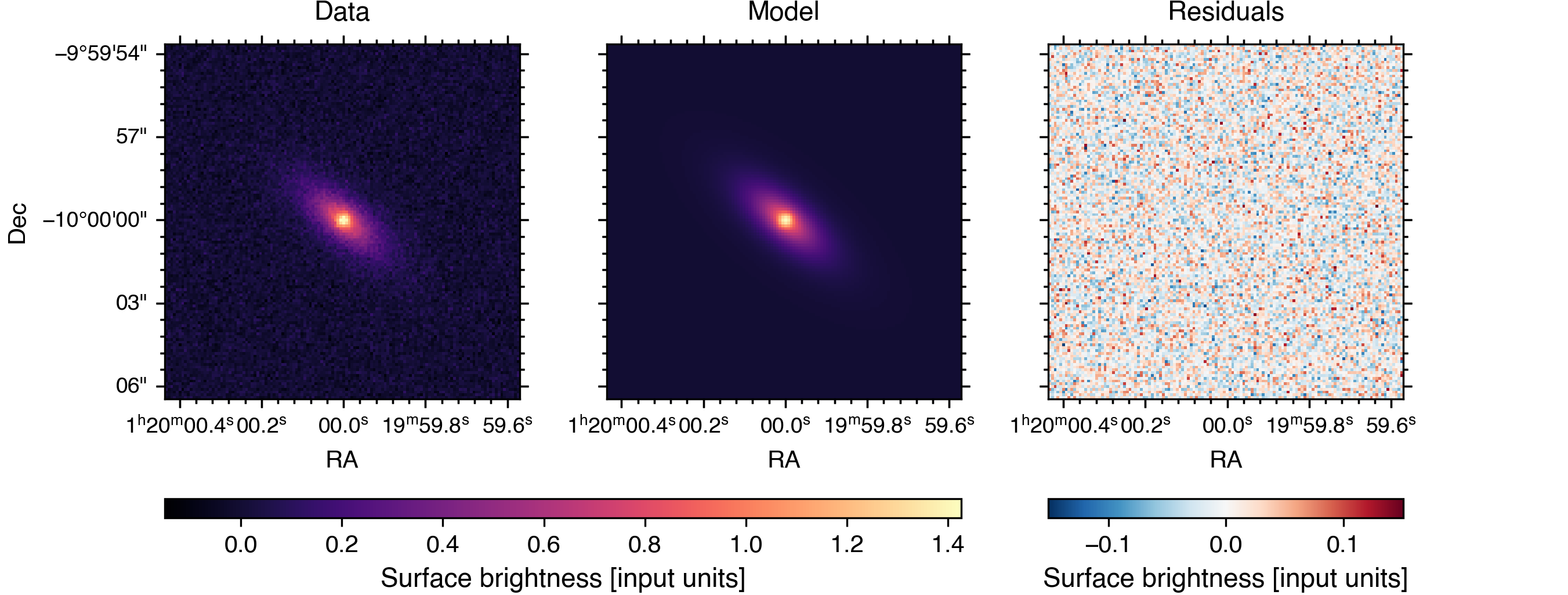
Comparison plot showing the data, model, and residuals for the fitted galaxy.

Note

By default, socca uses the best-fit parameters (i.e. those maximizing the posterior probability) to generate the model image shown in the comparison plot. In the case of strong parameter degeneracies, it is however more appropriate to consider the model obtained by marginalizing over the individual models generated for each sample in the posterior distribution. This can be achieved by passing the usebest=False argument to fit.plot.comparison(). Please note that, since this involves generating a model image for each sample in the posterior distribution, such an option is significantly more computationally expensive than using the best-fit parameters.

Additionally, it is possible to generate a corner plot of the posterior distributions of all free parameters simply by calling:

>>> fit.plot.corner()

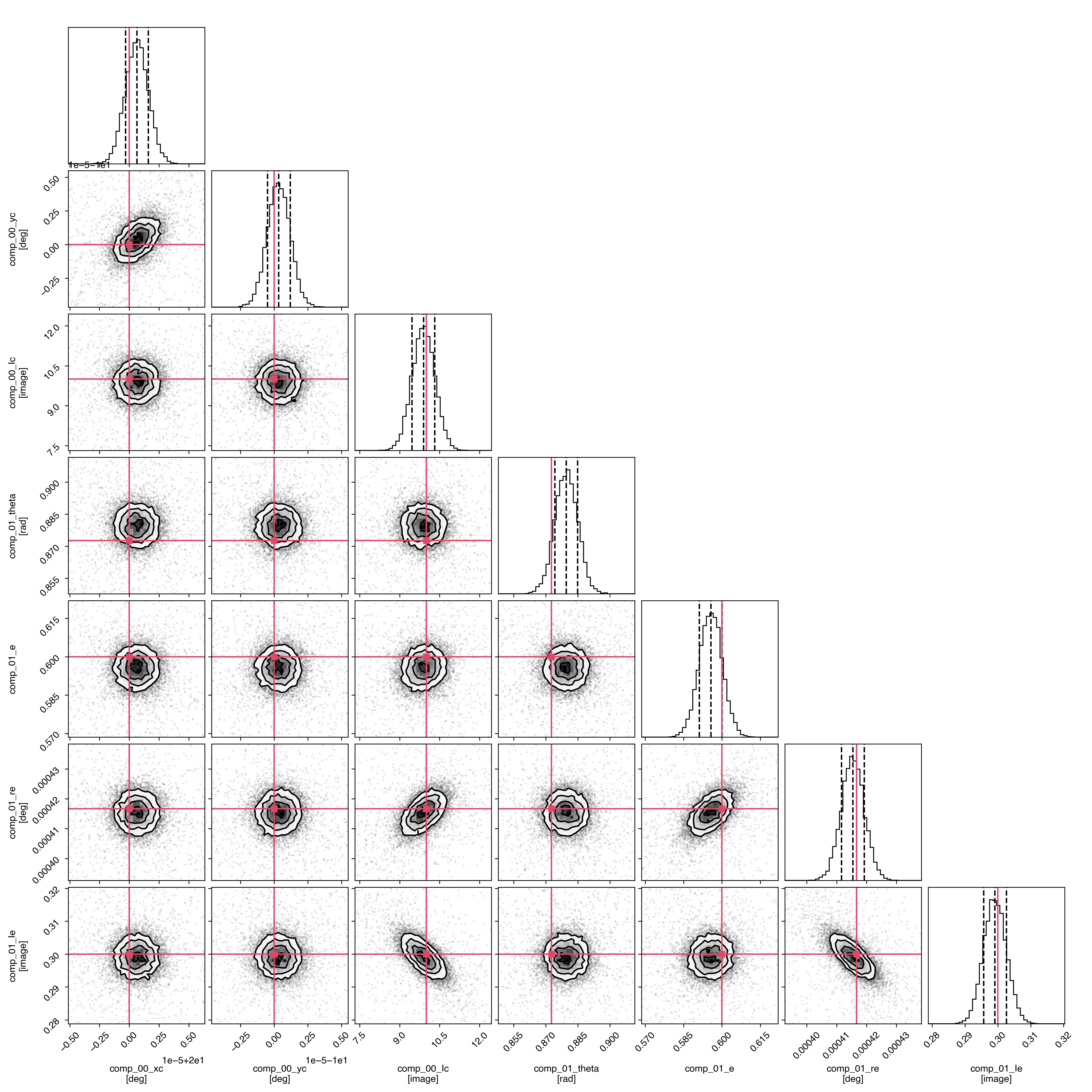
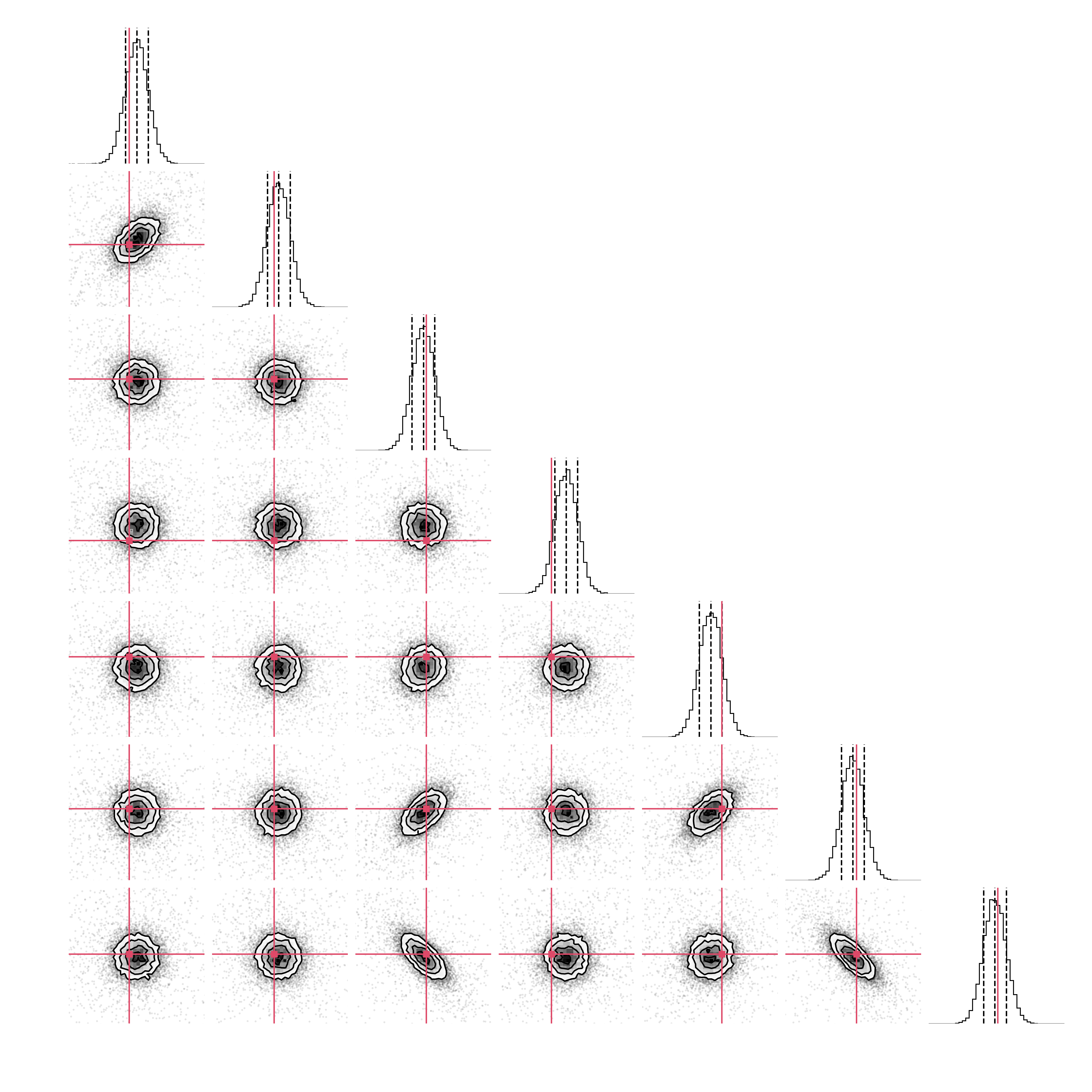
Corner plot showing the posterior distributions of the model parameters.

This is mostly a simple wrapper around corner.py that automatically configures the labels and ranges based on the model parameters and prior distributions. It is also possible to use it for visualising only a subset of the model components by passing a list of component names to the component argument as a list of strings (e.g. component=['comp_00'] to show only the first component added to the model), integer indices (e.g. component=[0]), or directly referring to the individual components (e.g. component=[point]).

By default, both the comparison and corner plots are displayed on screen. Passing the argument name="your/file/name/prefix" however allows for saving the figures to disk.

Finally, for a quick summary of the best-fit parameters and their uncertainties, you can use the parameters() method:

>>> fit.parameters()

Best-fit parameters
========================================

comp_00
-------
xc :  2.0000E+01 [+9.4877E-07/-9.6246E-07]
yc : -1.0000E+01 [+8.6032E-07/-8.3115E-07]
Ic :  9.8960E+00 [+4.2454E-01/-4.2952E-01]

comp_01
-------
theta :  8.7960E-01 [+5.3261E-03/-5.2986E-03]
e     :  5.9568E-01 [+4.3743E-03/-4.5214E-03]
re    :  4.1541E-04 [+3.8318E-06/-3.7940E-06]
Ie    :  2.9910E-01 [+3.5399E-03/-3.3804E-03]

The output shows the weighted median (50th percentile) as the best-fit value for each parameter of the combined model, along with the associated uncertainties derived from the 16th and 84th percentiles.